fcaR: Formal Concept Analysis with R
A comprehensive R package for Formal Concept Analysis, including logic handling and visualization.
Motivation
NoteWhy develop an
R package for FCA?
R, together with Python, are the two most widely used programming languages in Machine Learning and Data Science.- In
Rthere are already libraries for association rule mining that have become standard:arules. - There is no library in
Rthat implements the basic ideas and functions of FCA and allows them to be used seamlessly in other contexts.
History & Applications
TipHistory of FCA
- Port-Royal logic (traditional logic): formal notion of concept, Arnauld A., Nicole P. (1662): concept = extent (objects) + intent (attributes).
- G. Birkhoff (1940s): work on lattices and related mathematical structures, emphasizes applicational aspects of lattices in data analysis.
- Barbut M., Monjardet B.: Ordre et classiffication (1970).
- Wille R.: Restructuring lattice theory (1982).
- Ganter B., Wille R.: Formal Concept Analysis (Springer, 1999).
ImportantApplications of FCA
- Knowledge extraction
- Clustering and classification
- Machine learning
- Concepts, ontologies
- Rules, association rules, attribute implications
The fcaR library
The package is in a stable phase in a repository on Github and on CRAN.
- Unit tests & Vignettes with demos
- Status:
- lifecycle: stable
- CRAN version: 1.6.0

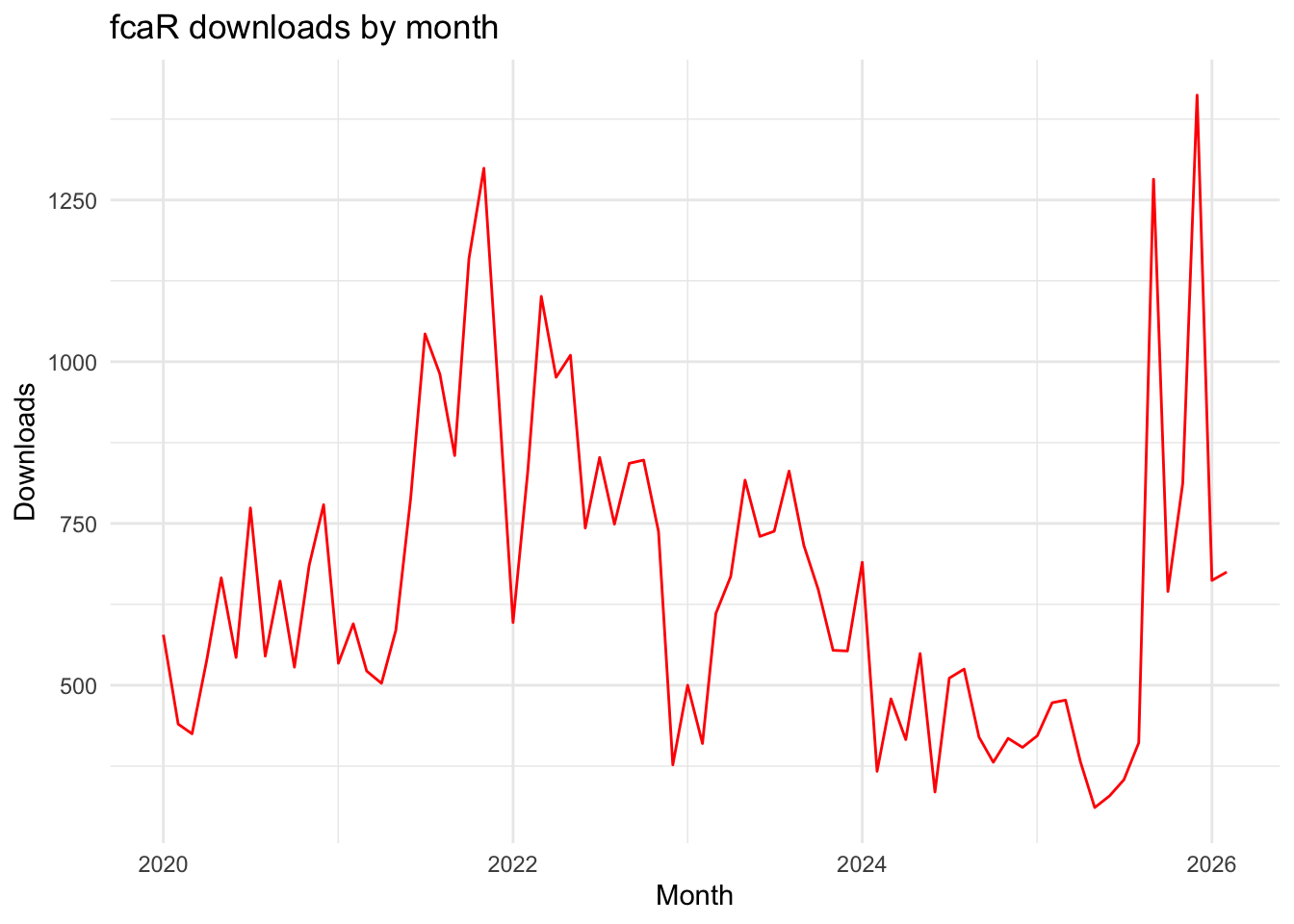
Live CRAN Downloads
Total fcaR CRAN downloads: 48,572
Installation
- Install R for your operating system: CRAN and (optional) RStudio.
- (Within R) Install
fcaR:
install.packages("fcaR")
TipWhere to find help
Visit the official fcaR pkgdown repository for references, articles, and advanced uses.
Part 0: Introduction
We will show some of the main methods of Formal Concept Analysis using the data structures of the fcaR package. We follow the discourse of Conceptual Exploration - B. Ganter, S. Obiedkov - 2016.
Structure of fcaR
The fcaR package provides data structures which allow the user to work seamlessly with formal contexts and sets of implications. Three basic objects will be used:
FormalContext: Encapsulates the definition of a formal context (G, M, I), being G the set of objects, M the set of attributes and I the (fuzzy) relationship matrix.ImplicationSet: Represents a set of implications (rules) over a specific formal context.Set: A class for storing variables (attributes or objects) efficiently.
By taking advantage of R’s Object Oriented Programming (R6), all knowledge (concepts, implications, etc.) is safely stored inside the formal context object itself. Under the hood, fcaR mixes R’s vectorization capabilities with fast C/C++ code for the algorithmic bottlenecks.
Part I: The Formal Context
FCA provides methods to describe the relationship between a set of objects G and a set of attributes M.
We show the main methods of FCA using the main functionalities and data structures of the fcaR package.
Formal contexts
The first step when using the fcaR package to analyse a formal context is to create a variable of class FormalContext which will store all the information related to the context.
We use the Formal Context, \mathbf{ K} := (G, M, I) about planets:
Wille R (1982). “Restructuring Lattice Theory: An Approach Based on Hierarchies of Concepts.” In Ordered Sets, pp. 445–470. Springer.
We load the fcaR package by:
Code
library(fcaR)- Visualizing the dataset
| small | medium | large | near | far | moon | no_moon | |
|---|---|---|---|---|---|---|---|
| Mercury | 1 | 0 | 0 | 1 | 0 | 0 | 1 |
| Venus | 1 | 0 | 0 | 1 | 0 | 0 | 1 |
| Earth | 1 | 0 | 0 | 1 | 0 | 1 | 0 |
| Mars | 1 | 0 | 0 | 1 | 0 | 1 | 0 |
| Jupiter | 0 | 0 | 1 | 0 | 1 | 1 | 0 |
| Saturn | 0 | 0 | 1 | 0 | 1 | 1 | 0 |
| Uranus | 0 | 1 | 0 | 0 | 1 | 1 | 0 |
| Neptune | 0 | 1 | 0 | 0 | 1 | 1 | 0 |
| Pluto | 1 | 0 | 0 | 0 | 1 | 1 | 0 |
- Creating a variable
fc_planets
Code
fc_planets <- FormalContext$new(planets)
fc_planets
FormalContext with 9 objects and 7 attributes.
small medium large near far moon no_moon
Mercury X X X
Venus X X X
Earth X X X
Mars X X X
Jupiter X X X
Saturn X X X
Uranus X X X
Neptune X X X
Pluto X X X fc_planets is a R variable which stores the formal context \mathbf{ K} but also, all the knowledge related with the data inside:
- the attributes M,
- the objects G,
- the incidence relation
- the concepts (when they are computed)
- the implications (when they are computed)
- etc.
Help: fcaR for your .tex documents:
Code
fc_planets$to_latex(
    caption = "Planets dataset.",
    label = "tab:planets"
)
\begin{table} \caption{Planets dataset.}\label{tab:planets} \centering \begin{tabular}{r|ccccccc}
& $\mathrm{small}$ & $\mathrm{medium}$ & $\mathrm{large}$ & $\mathrm{near}$ & $\mathrm{far}$ & $\mathrm{moon}$ & $\mathrm{no\_moon}$\\
\hline
$\mathrm{Mercury}$ & $\times$ & & & $\times$ & & & $\times$ \\
$\mathrm{Venus}$ & $\times$ & & & $\times$ & & & $\times$ \\
$\mathrm{Earth}$ & $\times$ & & & $\times$ & & $\times$ & \\
$\mathrm{Mars}$ & $\times$ & & & $\times$ & & $\times$ & \\
$\mathrm{Jupiter}$ & & & $\times$ & & $\times$ & $\times$ & \\
$\mathrm{Saturn}$ & & & $\times$ & & $\times$ & $\times$ & \\
$\mathrm{Uranus}$ & & $\times$ & & & $\times$ & $\times$ & \\
$\mathrm{Neptune}$ & & $\times$ & & & $\times$ & $\times$ & \\
$\mathrm{Pluto}$ & $\times$ & & & & $\times$ & $\times$ &
\end{tabular}
\end{table}which gives something like:
| small | medium | large | near | far | moon | no_moon | |
|---|---|---|---|---|---|---|---|
| Mercury | x | x | x | ||||
| Venus | x | x | x | ||||
| Earth | x | x | x | ||||
| Mars | x | x | x | ||||
| Jupiter | x | x | x | ||||
| Saturn | x | x | x | ||||
| Uranus | x | x | x | ||||
| Neptune | x | x | x | ||||
| Pluto | x | x | x |
fc_planets can be plotted (in gray scale for fuzzy datasets)
Code
fc_planets$plot()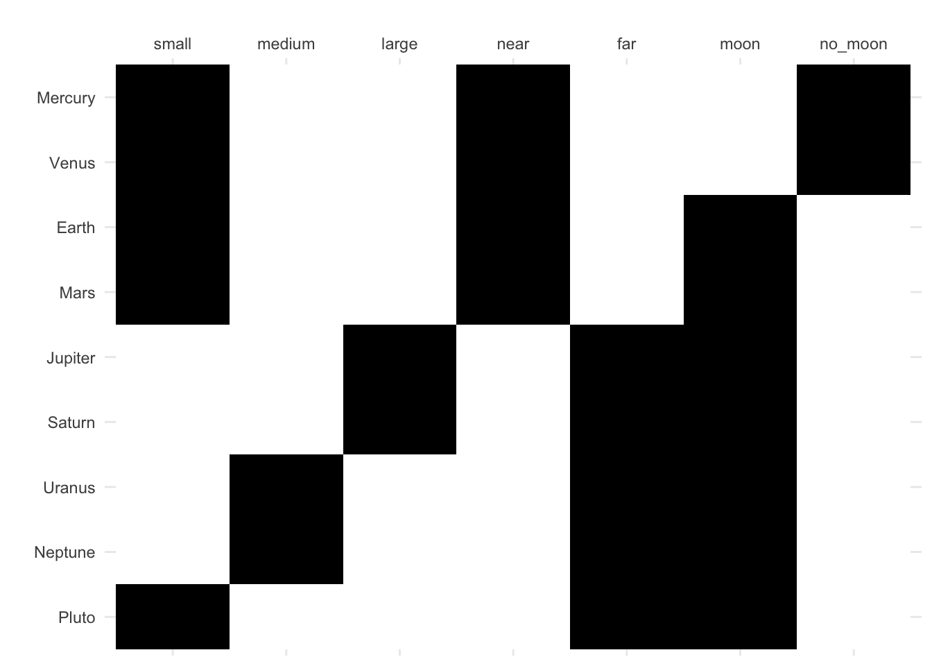
fc_planets can be saved or loaded in a file
Code
fc_planets$save(filename = "./fc_planets.rds")
fcnew <- FormalContext$new("./fc_planets.rds")
fcnew
FormalContext with 9 objects and 7 attributes.
small medium large near far moon no_moon
Mercury 1 0 0 1 0 0 1
Venus 1 0 0 1 0 0 1
Earth 1 0 0 1 0 1 0
Mars 1 0 0 1 0 1 0
Jupiter 0 0 1 0 1 1 0
Saturn 0 0 1 0 1 1 0
Uranus 0 1 0 0 1 1 0
Neptune 0 1 0 0 1 1 0
Pluto 1 0 0 0 1 1 0 Basic methods
Derivation operators
Functions intent() (\equiv^{\uparrow}) and extent() (\equiv^{\downarrow}) are designed to perform the corresponding operations:
A^{\uparrow} := \{m\in M : (g,m)\in I,\, \forall g\in A\} B^{\downarrow} := \{g\in G : (g,m)\in I,\, \forall m\in B\}
Example:
To compute \{{\rm Mars}, {\rm Earth}\}^{\uparrow}:
Code
set_objects <- Set$new(fc_planets$objects)
set_objects$assign(Mars = 1, Earth = 1)
fc_planets$intent(set_objects)
{small, near, moon}To compute \{{\rm medium}, {\rm far}\}^{\downarrow}:
Code
set_attributes <- Set$new(fc_planets$attributes)
set_attributes$assign(medium = 1, far = 1)
fc_planets$extent(set_attributes)
{Uranus, Neptune}This pair of mappings is a Galois connection.
The composition of intent and extent is the closure of a set of attributes.
Closures
To compute \{{\rm medium}\}^{\downarrow\uparrow}:
Code
# Compute the closure of S
set_attributes1 <- Set$new(fc_planets$attributes)
set_attributes1$assign(medium = 1)
MyClosure <- fc_planets$closure(set_attributes1)
MyClosure
{medium, far, moon}This means that all planets which have the attributes medium have far and moon in common.
The function $is_closed() allows us to know if a set of attributes is closed.
Code
set_attributes2 <- Set$new(attributes = fc_planets$attributes)
set_attributes2$assign(moon = 1, large = 1, far = 1)
set_attributes2
{large, far, moon}Code
# Is it closed?
fc_planets$is_closed(set_attributes2)
[1] TRUECode
set_attributes3 <- Set$new(attributes = fc_planets$attributes)
set_attributes3$assign(small = 1, far = 1)
set_attributes3
{small, far}Code
# Is it closed?
fc_planets$is_closed(set_attributes3)
[1] FALSEClarification and Reduction
Methods to simplify the context by removing redundancies, while preserving the structural knowledge.
clarify(): removes duplicated attributes and objects (columns and rows in the original matrix).reduce(): uses closures to remove dependent attributes, but only on binary formal contexts.
Code
# We clone the context just to keep a copy
fc_planetscopy <- fc_planets$clone()
fc_planetscopy$clarify(TRUE)
FormalContext with 5 objects and 7 attributes.
small medium large near far moon no_moon
Pluto X X X
[Mercury, Venus] X X X
[Earth, Mars] X X X
[Jupiter, Saturn] X X X
[Uranus, Neptune] X X X Code
fc_planetscopy$reduce(TRUE)FormalContext with 5 objects and 7 attributes.
small medium large near far moon no_moon
Pluto X X X
[Mercury, Venus] X X X
[Earth, Mars] X X X
[Jupiter, Saturn] X X X
[Uranus, Neptune] X X X Note that merged attributes or objects are stored in the new formal context by using squared brackets to unify them, e.g. [Mercury, Venus]
Part II: Concepts & The Lattice
Concepts
\big(\{{\rm Jupiter}, {\rm Saturn}, {\rm Uranus}, {\rm Neptune}, {\rm Pluto}\},\{{\rm far}, {\rm moon}\}\big) is a concept. It is a maximal cluster.
| small | medium | large | near | far | moon | no_moon | |
|---|---|---|---|---|---|---|---|
| Mercury | x | x | x | ||||
| Venus | x | x | x | ||||
| Earth | x | x | x | ||||
| Mars | x | x | x | ||||
| Jupiter | x | x | x | ||||
| Saturn | x | x | x | ||||
| Uranus | x | x | x | ||||
| Neptune | x | x | x | ||||
| Pluto | x | x | x |
Note: concepts for your .tex documents:
Code
fc_planets$concepts$to_latex()Computing concepts
We use the function $find_concepts()
Computing all the concepts from formal context of planets:
Code
fc_planets$find_concepts()
fc_planets$concepts
A set of 12 concepts:
1: ({}, {small, medium, large, near, far, moon, no_moon})
2: ({Mercury, Venus, Earth, Mars, Jupiter, Saturn, Uranus, Neptune, Pluto}, {})
3: ({Uranus, Neptune}, {medium, far, moon})
4: ({Jupiter, Saturn}, {large, far, moon})
5: ({Mercury, Venus}, {small, near, no_moon})
6: ({Mercury, Venus, Earth, Mars}, {small, near})
7: ({Earth, Mars}, {small, near, moon})
8: ({Mercury, Venus, Earth, Mars, Pluto}, {small})
9: ({Pluto}, {small, far, moon})
10: ({Earth, Mars, Pluto}, {small, moon})
11: ({Jupiter, Saturn, Uranus, Neptune, Pluto}, {far, moon})
12: ({Earth, Mars, Jupiter, Saturn, Uranus, Neptune, Pluto}, {moon})Code
# First 6 concepts
head(fc_planets$concepts)
A set of 6 concepts:
1: ({}, {small, medium, large, near, far, moon, no_moon})
2: ({Mercury, Venus, Earth, Mars, Jupiter, Saturn, Uranus, Neptune, Pluto}, {})
3: ({Uranus, Neptune}, {medium, far, moon})
4: ({Jupiter, Saturn}, {large, far, moon})
5: ({Mercury, Venus}, {small, near, no_moon})
6: ({Mercury, Venus, Earth, Mars}, {small, near})Code
# The first concept
firstconcept <- fc_planets$concepts[1]
firstconcept
A set of 1 concepts:
1: ({}, {small, medium, large, near, far, moon, no_moon})Visualizing the Concept Lattice
A fundamental component of Formal Concept Analysis is the visualization of the data hierarchy using Hasse diagrams.
Code
# Plot the Hasse diagram of the concept lattice
fc_planets$concepts$plot()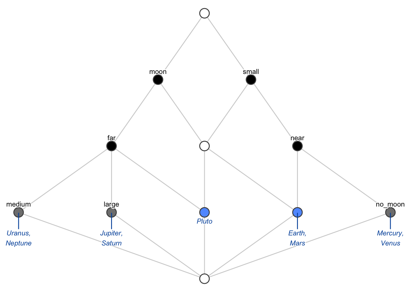
Click to see advanced layout settings!
Note
fcaR layout adapts automatically, but you can explicitly use different labeling modes via the mode argument: mode = "reduced" (default), mode = "full" (all attributes/objects), or mode = "empty" (structure only, great for large lattices).
Code
# Full labeling mode
fc_planets$concepts$plot(mode = "full")
Notable elements (Irreducibles)
In a complete lattice, an element is called supremum-irreducible or join-irreducible if it cannot be written as the supremum of other elements and infimum-irreducible or meet-irreducible if it can not be expressed as the infimum of other elements.
The irreducible elements with respect to join (supremum) and meet (infimum) can be extracted from a given concept lattice:
Code
fc_planets$concepts$join_irreducibles()A set of 5 concepts:
1: ({Uranus, Neptune}, {medium, far, moon})
2: ({Jupiter, Saturn}, {large, far, moon})
3: ({Mercury, Venus}, {small, near, no_moon})
4: ({Earth, Mars}, {small, near, moon})
5: ({Pluto}, {small, far, moon})Code
fc_planets$concepts$meet_irreducibles()A set of 7 concepts:
1: ({Uranus, Neptune}, {medium, far, moon})
2: ({Jupiter, Saturn}, {large, far, moon})
3: ({Mercury, Venus}, {small, near, no_moon})
4: ({Mercury, Venus, Earth, Mars}, {small, near})
5: ({Mercury, Venus, Earth, Mars, Pluto}, {small})
6: ({Jupiter, Saturn, Uranus, Neptune, Pluto}, {far, moon})
7: ({Earth, Mars, Jupiter, Saturn, Uranus, Neptune, Pluto}, {moon})Part III: Implications & Simplification
Computing
find_implications(): the function to extract the canonical basis of implications and the concept lattice using the NextClosure algorithm
It stores both a ConceptLattice and an ImplicationSet objects internally in the FormalContext variable.
Code
fc_planets$find_implications()Manipulating and Filtering Rules
The computed implications are:
Code
fc_planets$implicationsImplication set with 10 implications.
Rule 1: {no_moon} -> {small, near}
Rule 2: {far} -> {moon}
Rule 3: {near} -> {small}
Rule 4: {large} -> {far, moon}
Rule 5: {medium} -> {far, moon}
Rule 6: {medium, large, far, moon} -> {small, near, no_moon}
Rule 7: {small, near, moon, no_moon} -> {medium, large, far}
Rule 8: {small, near, far, moon} -> {medium, large, no_moon}
Rule 9: {small, large, far, moon} -> {medium, near, no_moon}
Rule 10: {small, medium, far, moon} -> {large, near, no_moon}Implications can be read by sub-setting (the same as in the standard R language vectors):
Code
fc_planets$implications[3]Implication set with 1 implications.
Rule 1: {near} -> {small}Code
fc_planets$implications[1:4]Implication set with 4 implications.
Rule 1: {no_moon} -> {small, near}
Rule 2: {far} -> {moon}
Rule 3: {near} -> {small}
Rule 4: {large} -> {far, moon}Code
fc_planets$implications[c(1:4, 3)]Implication set with 5 implications.
Rule 1: {no_moon} -> {small, near}
Rule 2: {far} -> {moon}
Rule 3: {near} -> {small}
Rule 4: {large} -> {far, moon}
Rule 5: {near} -> {small}Filtering Rules based on Conditions
You can easily filter the rules using fcaR’s intuitive semantic filtering commands (filter(), lhs_has(), rhs_has()). These are designed to feel like native data manipulation verbs!
For example, let’s keep only the rules that have a Left-Hand Side (LHS) with more than 1 attribute:
Code
# Filter rules with LHS size > 1
filtered_imps <- fc_planets$implications %>%
  filter(lhs_size > 1)
filtered_imps
Implication set with 5 implications.
Rule 1: {medium, large, far, moon} -> {small, near, no_moon}
Rule 2: {small, near, moon, no_moon} -> {medium, large, far}
Rule 3: {small, near, far, moon} -> {medium, large, no_moon}
Rule 4: {small, large, far, moon} -> {medium, near, no_moon}
Rule 5: {small, medium, far, moon} -> {large, near, no_moon}Or combining numeric conditions: Keep implications where LHS has only 1 attribute BUT RHS has more than 1 attribute:
Code
fc_planets$implications %>%
  filter(lhs_size == 1, rhs_size > 1)
Implication set with 3 implications.
Rule 1: {no_moon} -> {small, near}
Rule 2: {large} -> {far, moon}
Rule 3: {medium} -> {far, moon}We can also do Semantic Filtering directly on the traits! What if we want to find all rules that explicitly imply a planet has a moon?
Code
# Semantic filtering
fc_planets$implications %>%
  filter(rhs_has("moon"))
Implication set with 3 implications.
Rule 1: {far} -> {moon}
Rule 2: {large} -> {far, moon}
Rule 3: {medium} -> {far, moon}Cardinality & Sizes
- the number of implications is computed using
fc_planets$implications$cardinality() - the number of attributes for each implication is computed using
fc_planets$implications$size()
Code
fc_planets$implications$cardinality()[1] 10Code
sizes <- fc_planets$implications$size()
head(sizes)
LHS RHS
[1,] 1 2
[2,] 1 1
[3,] 1 1
[4,] 1 2
[5,] 1 2
[6,] 4 3Code
colMeans(sizes)LHS RHS
2.5 2.3 Help: … for your .tex documents:
Code
fc_planets$implications$to_latex()\begin{longtable*}{rrcl}
1: &\left\{\mathrm{no\_moon}\right\}&\ensuremath{\Rightarrow}&\left\{\mathrm{small}, \mathrm{near}\right\}\\
2: &\left\{\mathrm{far}\right\}&\ensuremath{\Rightarrow}&\left\{\mathrm{moon}\right\}\\
3: &\left\{\mathrm{near}\right\}&\ensuremath{\Rightarrow}&\left\{\mathrm{small}\right\}\\
4: &\left\{\mathrm{large}\right\}&\ensuremath{\Rightarrow}&\left\{\mathrm{far}, \mathrm{moon}\right\}\\
5: &\left\{\mathrm{medium}\right\}&\ensuremath{\Rightarrow}&\left\{\mathrm{far}, \mathrm{moon}\right\}\\
6: &\left\{\mathrm{medium}, \mathrm{large}, \mathrm{far}, \mathrm{moon}\right\}&\ensuremath{\Rightarrow}&\left\{\mathrm{small}, \mathrm{near}, \mathrm{no\_moon}\right\}\\
7: &\left\{\mathrm{small}, \mathrm{near}, \mathrm{moon}, \mathrm{no\_moon}\right\}&\ensuremath{\Rightarrow}&\left\{\mathrm{medium}, \mathrm{large}, \mathrm{far}\right\}\\
8: &\left\{\mathrm{small}, \mathrm{near}, \mathrm{far}, \mathrm{moon}\right\}&\ensuremath{\Rightarrow}&\left\{\mathrm{medium}, \mathrm{large}, \mathrm{no\_moon}\right\}\\
9: &\left\{\mathrm{small}, \mathrm{large}, \mathrm{far}, \mathrm{moon}\right\}&\ensuremath{\Rightarrow}&\left\{\mathrm{medium}, \mathrm{near}, \mathrm{no\_moon}\right\}\\
10: &\left\{\mathrm{small}, \mathrm{medium}, \mathrm{far}, \mathrm{moon}\right\}&\ensuremath{\Rightarrow}&\left\{\mathrm{large}, \mathrm{near}, \mathrm{no\_moon}\right\}\\
\end{longtable*}Redundancy & Simplification
Code
# Before simplification: Check mean size
sizes <- fc_planets$implications$size()
colMeans(sizes)

# Let's apply Equivalence Rules!
fc_planets$implications$apply_rules(
    rules = c("composition", "generalization", "simplification")
)

# Simplified implications are much cleaner!
fc_planets$implicationsValidity
We can see if an ImplicationSet holds in a FormalContext by using the %holds_in% operator.
For instance, we can check that the first implication so far in the Duquenne-Guigues basis holds in the planets formal context:
Code
imp1 <- fc_planets$implications[1]
imp1
Implication set with 1 implications.
Rule 1: {no_moon} -> {small, near}Code
imp1 %holds_in% fc_planets[1] TRUEInteractive Exercises
Time to put what we’ve learned into practice! Try to solve these questions using the fc_planets object.
If you are stuck, you can expand the solution block.
Exercise 1: Intents
Compute the intent of the object Earth. Then, compute the intent of {Earth, Mars, Mercury}.
Expected Output:
Intent for Earth:{small, near, moon}Intent for Earth, Mars, Mercury:{small, near}Exercise 2: Extents
Compute the extent of large and {far, large}. Save the result in variables e1 and e2. What happens if you compute the intent of e1 and e2? What are you computing here?
Expected Output:
Extent for large:{Jupiter, Saturn}Extent for {far, large}:{Jupiter, Saturn}
If we compute the intents, we are computing the closures!{large, far, moon}{large, far, moon}Exercise 3: Concepts
Using the att_concept() and obj_concept() shortcut functions, find: 1. The highest concept that has moon. 2. The lowest concept that has Pluto.
Expected Output:
({Earth, Mars, Jupiter, Saturn, Uranus, Neptune, Pluto}, {moon})({Pluto}, {small, far, moon})Exercise 4: Playing with Random Contexts (New!)
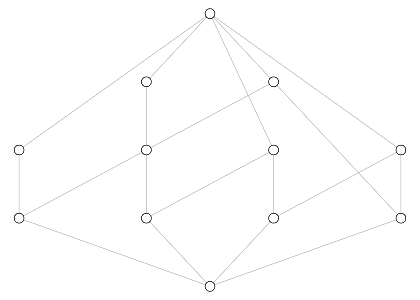
fcaR has a built-in generator for realistic synthetic datasets! Can you generate a random context of 10 objects and 5 attributes with a 0.3 density, and then plot its concept lattice using mode = "empty"?
Expected Output Plot:
Extra: Advanced Topics
Warning
The following sections cover advanced features of the fcaR package (Sublattices, Protoconcepts, Entailment, etc.) which are beyond the scope of strictly basic 1-hour usage, but are very useful for research.
Concept support
The support of a concept \langle A, B\rangle (A is the extent of the concept and B is the intent) is the cardinality (relative) of the extent - number of objects of the extent.
supp(\langle A, B\rangle)=\frac{|A|}{|G|}
We use the function: $support()
Code
fc_planets$concepts$support() [1] 1.0000000 0.7777778 0.5555556 0.2222222 0.2222222 0.5555556 0.3333333
[8] 0.1111111 0.4444444 0.2222222 0.2222222 0.0000000️ The support of itemsets and concepts is used to mine all the knowledge in the dataset: Algorithm Titanic - computing iceberg concept lattices.
Sublattices
When the concept lattice is too large, it can be useful in certain occasions to just work with a sublattice of the complete lattice. To this end, we use the sublattice() function.
$sublattice(): find a sublattice of the complete lattice
For instance: Computing a sublattice of those concepts with support greater than the threshold
Code
fc_planets$conceptsA set of 12 concepts:
1: ({Mercury, Venus, Earth, Mars, Jupiter, Saturn, Uranus, Neptune, Pluto}, {})
2: ({Earth, Mars, Jupiter, Saturn, Uranus, Neptune, Pluto}, {moon})
3: ({Jupiter, Saturn, Uranus, Neptune, Pluto}, {far, moon})
4: ({Jupiter, Saturn}, {large, far, moon})
5: ({Uranus, Neptune}, {medium, far, moon})
6: ({Mercury, Venus, Earth, Mars, Pluto}, {small})
7: ({Earth, Mars, Pluto}, {small, moon})
8: ({Pluto}, {small, far, moon})
9: ({Mercury, Venus, Earth, Mars}, {small, near})
10: ({Mercury, Venus}, {small, near, no_moon})
11: ({Earth, Mars}, {small, near, moon})
12: ({}, {small, medium, large, near, far, moon, no_moon})Code
# Compute index of interesting concepts - using support
idx <- which(fc_planets$concepts$support() > 0.5)
# Build the sublattice
sublattice <- fc_planets$concepts$sublattice(idx)
sublattice
sublattice$plot()

# Compute index of interesting concepts - using indexes
idx <- c(8, 9, 10) # concepts 8, 9 and 10
# Build the sublattice
sublattice <- fc_planets$concepts$sublattice(idx)
sublattice
sublattice$plot()
Hierarchy
That is: Subconcepts, superconcepts, infimum and supremum
Given a concept, we can compute all its subconcepts and all its superconcepts.
For instance, find all the subconcepts and superconcepts of the concept number 5 in the list of concepts.
Code
C <- fc_planets$concepts[5]
C
# Its subconcepts:
fc_planets$concepts$subconcepts(C)
# And its superconcepts:
fc_planets$concepts$superconcepts(C)
The same, for supremum and infimum of a set of concetps.
To find the supremum and the infimum of the concepts 5,6,7.
Code
# A list of concepts
C <- fc_planets$concepts[5:7]
C

# Supremum of the concepts in C
fc_planets$concepts$supremum(C)
# Infimum of the concepts in C
fc_planets$concepts$infimum(C)
Standard Context
The standard context is ({\cal J}, {\cal M}, \leq), where \cal J is the set of join-irreducible concepts and \cal M are the meet-irreducible ones.
standardize() is the function to compute the standard context.
Note: objects are now named J1, J2… and attributes are M1, M2…, from join and meet
Code
fc_planetscopy <- fc_planets$clone()
fc_planetscopy$find_concepts()
fc_planetscopy$standardize()
FormalContext with 5 objects and 7 attributes.
M1 M2 M3 M4 M5 M6 M7
J1 X X X
J2 X X X
J3 X X X
J4 X X X
J5 X X X Entailment
Imp1 %entails% Imp2 - Imp2 can be derived (logical consequence) of Imp1
Code
fc_planets$find_implications()
imps <- fc_planets$implications
imps2 <- fc_planets$implications$clone()
imps2$apply_rules(c("simp", "rsimp"))
imps %entails% imps2
[,1] [,2] [,3] [,4] [,5] [,6] [,7] [,8] [,9] [,10]
[1,] TRUE TRUE TRUE TRUE TRUE TRUE TRUE TRUE TRUE TRUECode
imps2 %entails% imps [,1] [,2] [,3] [,4] [,5] [,6] [,7] [,8] [,9] [,10]
[1,] TRUE TRUE TRUE TRUE TRUE TRUE TRUE TRUE TRUE TRUEEquivalence
Imp1 %~% Imp2 - Are Imp1 and Imp2 equivalent?
Code
imps %~% imps2[1] TRUECode
imps %~% imps2[1:3][1] FALSE